SeaHawk/HawkEye ▸ Data Collection & Processing
The goal of the SeaHawk mission was to demonstrate as a Proof of Concept, whether it is possible to obtain high quality, high resolution (~100m) ocean color imagery using a low-cost miniature ocean color sensor (HawkEye) carried aboard a CubeSat (SeaHawk). Under the terms of the formal NASA/HQ Space Act Agreement (2017) between NASA and the University of North Carolina/Wilmington ), NASA provides services for the collection, processing, calibration, validation, archival and distribution of the HawkEye data. The diagram below depicts all the interfaces involved in supporting the SeaHawk Mission which despite its small size, requires that all the same functions be performed as one would expect in the typical Earth observing satellite mission.

The HawkEye instrument collects images that are 1800 pixels x 6000 lines over 100 seconds which at the current altitude (~585km) provides a scene that is approximately 200 km across track and 600 km along track. Each image is approximately 100MB in size and the storage capacity onboard the spacecraft allows for 18 images (1.8GB) to be stored. SeaHawk has a miniature X-band transmitter that it uses to downlink the stored images as it passes over the NASA Near Earth Network receiving stations at Wallops Island, Virginia and the University of Alaska, Fairbanks and typically, we are able to schedule six or seven downlinks per week. Schedules for image collection and data downlinks are created to cover a 10-day period and we try and maximize the number of images collected between downlinks. Taking into consideration a number of other operational constraints, this allows us to anticipate collecting on average 100 images per week. Below is the map that was generated by our planning tool showing the images that were scheduled and data downlinks at both Wallops and Alaska for 21 June 2021, our first day of nominal operations.

Within minutes of the data being downlinked at the ground stations, the files are transferred to the Ocean Biology Processing Group's facility at NASA/Goddard where they are processed into Level-1a files and the special browse images that are used in the manual renavigation step that is described in the section on geolocation. Once the navigation adjustments are determined, each file is then submitted for processing to Level-2 and released for distribution via the OceanColor Web browser.
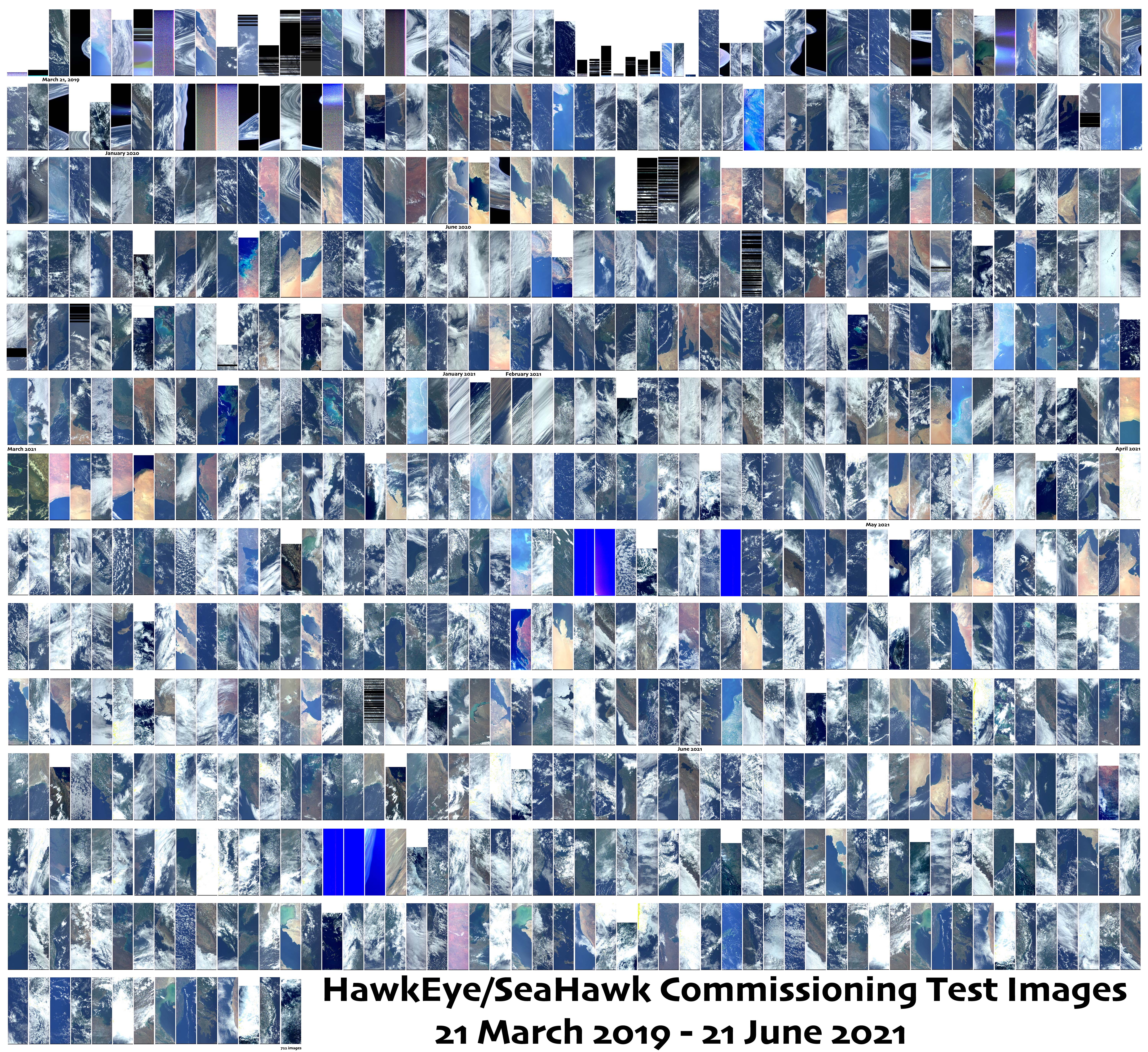
Over the course of the 2 ½ year commissioning phase of the mission, a number of different instrument configurations were tested to try and maximize the scientific quality of the images finally settling on a configuration on 16 April 2021 that was decided would be the default as we moved into nominal operations. The current calibration configuration that is used in our production system and that is provided in SeaDAS is optimized for data collected after this date. However, all data collected from the very first image that was collected on 21 March 2019 through the present day are available for download.
The Hawkeye instrument has been in orbit since December 3rd, 2018. Early in the mission life, an unstable attitude control resulted in the spacecraft tumbling between exposures, subjecting the optics and surfaces to direct solar illumination as well as pointing into the flight direction. Some loss of sensitivity in the blue bands has been noted, as well as apparent ablation of anti-reflection coatings on the exterior optical surfaces.
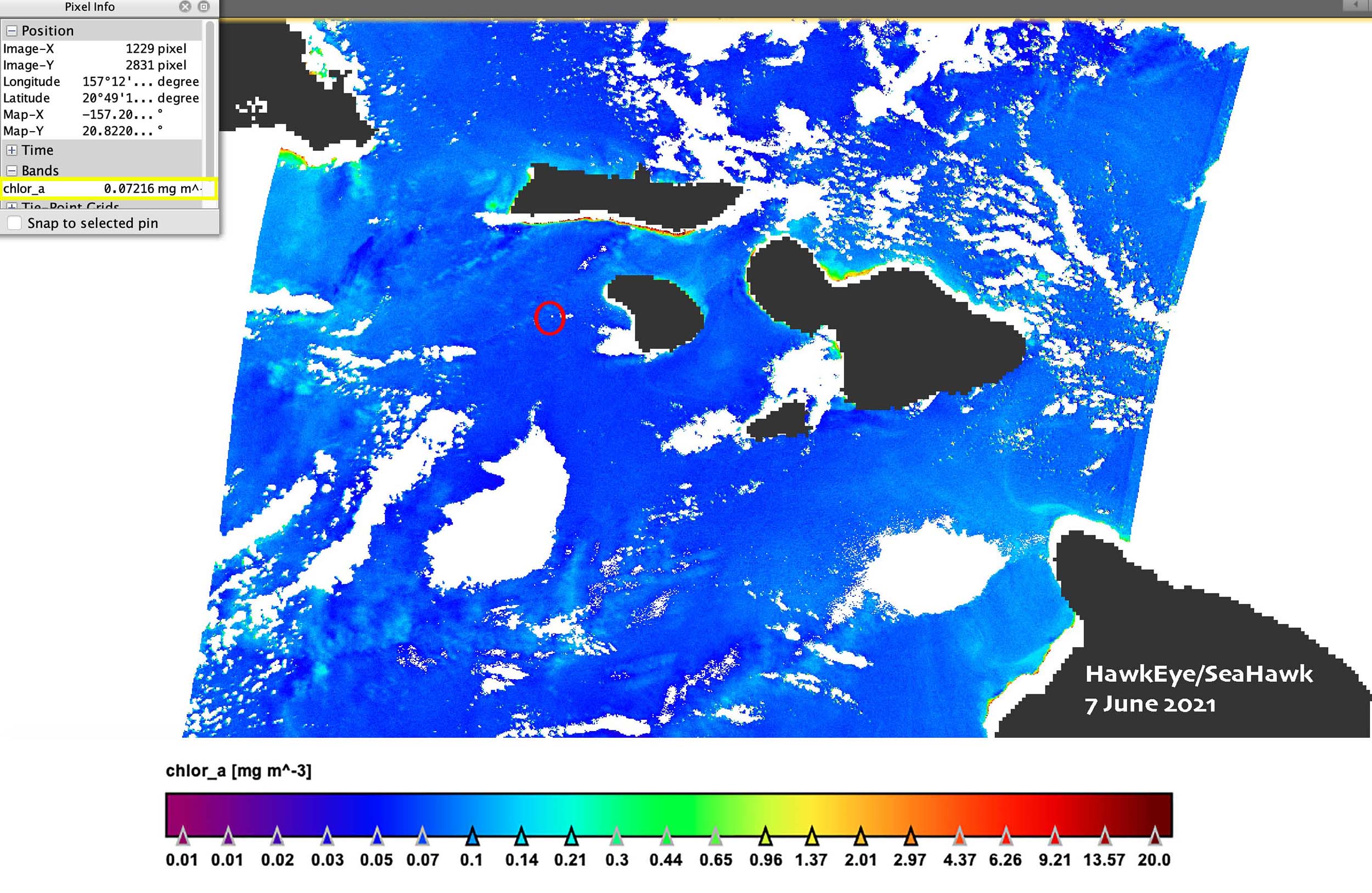
The HawkEye sensor has a band set similar to SeaWiFS and is capable of using the same Gordon and Wang (1994) approach for atmospheric correction. Unfortunately, as a result of this apparent ablation of the AR coating, the NIR bands suffer from a ghosting problem when there are bright targets (land, clouds) in the scene. This renders the use of the NIR bands in the atmospheric correction less than optimal. To avoid this issue affecting the operational products, the approach used for CZCS has been used.
This CZCS-like atmospheric correction uses a single aerosol model (instead of the 80 used in the current implementation of the GW94 approach) and the 670nm band to estimate the aerosol contribution with the assumption that the water-leaving signal is negligible. As it well known that the water-leaving signal at 670nm is often not negligible, especially in coastal and productive waters, a simple correction for estimating this contribution is employed. However, if there is a moderate to large water-leaving contribution, this correction will not be effective and the aerosol signal will be over estimated. This will result in an under estimate the Rrs which in turn will result in an over estimate of the chlorophyll concentration.
For most of the data collected by HawkEye, the results using the simplified CZCS-approach are quite good and comparable to coincident measurements by other satellite instruments. Below are two comparisons between HawkEye and the other sensors that we work with. The first is a qualitative comparison of the chlorophyll concentration estimate from HawkEye and OLCI on Sentinel-3A collected over the western Medeterranean Sea around Mallorca on May 29th, 2021. Both images were mapped to 300m resolution.
| HawkEye | OLCI-S3A |
|---|---|
 |
 |
| HawkEye | MODIS-Terra |
|---|---|
 |
 |
The ghosting effect is most evident in the NIR bands, so when these bands are used in the atmospheric correction as they are for the GW94 method, the ghosting will show up as an obvious artifact in the derived products.
| Lt_867 | Lt_670 | aot_867 |
|---|---|---|
 |
 |
 |
