This algorithm returns the skin sea surface temperature in units of °C. The long-wave infrared (LWIR) SST products make use of the 11 and 12 µm spectral bands aboard MODIS and VIIRS. The current LWIR algorithm is applicable for daytime and night time observations and is based on a modified version of the nonlinear SST algorithm of Walton et. al. (1998), most recently described in Kilpatrick et.al. (2015). The use of this algorithm provides product continuity between NASA’s current and future IR sensors and heritage Pathfinder SST from AVHRRs, thus enabling the generation of a 30+ year record of space based measurements of LWIR SST from polar orbiting satellites.
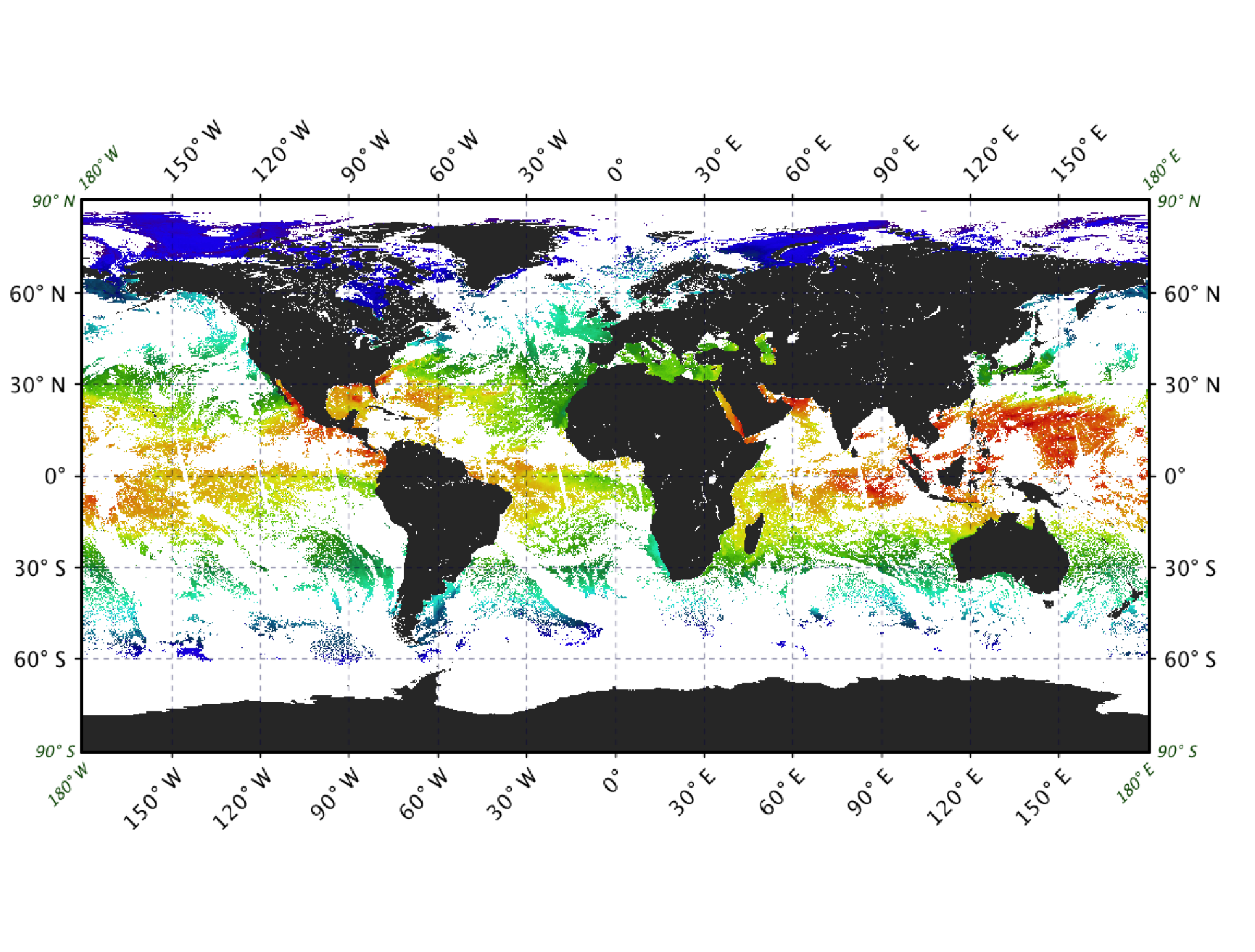
Figure 1 shows an example of global SST derived from one day of S-NPP VIIRS data taken during the sunlit part of each orbit.
Algorithm point of contact: Peter Minnett of the Rosenstiel School of Marine and Atmospheric Science (RSMAS) at the University of Miami.
The MODIS SST algorithm and quality assessment are the responsibility of the MODIS Science Team Lead for SST (currently P. Minnett of the Rosenstiel School of Marine and Atmospheric Science (RSMAS) at the University of Miami). In August 2018, the NASA VIIRS SST became an orphaned, unsupported product and, although the production at OBPG continues, users are advised to use VIIRS SST products with caution as the quality is no longer rigorously monitored by the SST science team.
NASA's standard processing and distribution of the SST products are performed using software developed by the Ocean Biology Processing Group (OB.DAAC/OBPG). The OB.DAAC generates Level-2 SST products using the Multi-Sensor Level-1 to Level-2 software (l2gen), which is the same software used to generate MODIS and VIIRS ocean color products. The TOA brightness temperatures used by the SST algorithm are derived from the measured calibrated radiances using Planck’s Equation convolved with the spectral response function of each band. To facilitate processing directly from the L1a files, and eliminate the need to archive the L1b at the OB.DAAC, l2gen uses a radiance to brightness temperature relationship table that is precomputed for the spectral response of each channel. These precomputed tables have been verified to produce identical brightness temperatures to those found in the standard L1b files and are stored locally and loaded during L2 processing at runtime.
Details of the SST processing implementation within l2gen are provided in this document. The description is valid for both the NASA standard products distributed by the OB.DAAC through the ocean color web and the products delivered to the Physical Oceanography DAAC, where the latter are subsequently repackaged for the Group for high resolution SST (GHRSST) distribution in L2p format. Historical documentation on the transition of MODIS SST processing from EOS MODAPS/DAAC/RSMAS to OB.DAAC in 2006 is available here.
The sea surface temperature measured by MODIS and VIIRS infrared radiometers is commonly referred to as the skin temperature of the ocean. This is because the radiance measured by infrared radiometers originates in the surface thermal skin layer of the ocean and not the body of water below as measured by in situ thermometers (Donlon et al., 2007). The thermal skin layer of the ocean is less than 1mm thick (Hanafin, 2002; Hanafin and Minnett, 2003; Wong and Minnett, 2018) and as a rule is cooler than the underlying water due to vertical heat flux, with the direction of flux typically from the ocean to the atmosphere. Three distinct processes impact near surface ocean temperature gradients: absorption of solar isolation, heat exchange with the atmosphere, and sub-surface turbulence. Generally, at night or when wind speeds are greater than ~6m/s the relationship between the skin temperature and the subsurface is often quite stable. It is under these conditions that validation and uncertainty estimates relative to sub-surface in situ buoys are typically reported. The relationship can however be very variable under conditions of high insolation, low wind speeds, and reduced sub-surface turbulence (Minnett, 2003; Ward, 2006). A more complete discussion of subsurface SST gradients and SST definitions and applications can be found here. The challenge of validating satellite skin SST measures for a climate data record, and the use of ship board radiometers for validation, can be found in Minnett (2010), Minnett and Corlett (2012) and Corlett et al., (2014).
The NASA objective in reprocessing of MODIS and VIIRS SST is to develop and apply, across multiple sensors, a consistent atmospheric correction algorithm and cloud detection to LWIR retrievals of skin SST, and provide known and predictable error and uncertainty characteristics of the skin SST products. The goal is inter-sensor continuity of LWIR SST retrievals and to extending the decades of SST measurements made by US sensors beginning with the AVHRR’s in the 1980’s to current MODIS and Suomi-NPP VIIRS sensors, and future JPSS VIIRS radiometers.
The current SST continuity algorithm is based on a modified version of the nonlinear SST algorithm (NLSST) of Walton et al. (1998) and uses empirical coefficients derived by regression of collocated in situ and satellite measurements. AVHRR Pathfinder SST and early versions of MODIS SST prior to R2014 (R2010 a.k.a. Collection 5 and 4) used monthly sets of coefficients for two different atmospheric regimes based on spectral brightness temperature difference as described by Kilpatrick et. al. (2001; 2015). Beginning with R2014, NASA skin SST products use month of year coefficients derived for distinct atmospheric regions based on latitude bands. R2014 and R2016 used 6 latitude bands in 20° intervals from 0° to 40°, and then a single large interval from 40° poleward in each hemisphere. The current MODIS R2019 skin SST products have coefficients for an additional 7th band above 60°N to better represent Arctic atmospheres (Kilpatrick et. al. 2019b; Jia, 2019; Jia & Minnett, 2020).
The base NLSST algorithm form was developed for use with the heritage NOAA/NASA AVHRR Pathfinder SST products and is described in detail in Kilpatrick et al. (2001). To extend the NLSST algorithm for optimum performance with the modern sensor design characteristics of MODIS and VIIRS, three additional algorithm terms were added to the base formulation. These new terms are related to (i) correcting for any potential residual imbalance between mirror sides, (ii) reducing any response versus scan angle (RVS) issues that may be present due to uncharacterized changes or degradation in mirror surfaces, and (iii) improving retrievals at the increasing path-lengths of MODIS and VIIRS towards the edges of the swaths.
The current algorithm for computing skin SST from measured LWIR brightness temperatures is shown below.
The coefficients aij are derived and continuously verified based on match-ups between the satellite brightness temperatures derived from the measured radiances and field measurements of sea surface temperature. As currently implemented, these coefficients are latitude band and time-dependent month of year. The coefficients are provided to l2gen through external files, which are in a columned ascii format of “sensor, month-start-day, month-end-day, latitude-start, latitude-end, ai0, ai1, ai2, ai3, ai4, ai5” the last several fields of each record contain internal diagnostic information and can be ignored. Coefficient sets are sensor-dependent. A link to the MODIS/Aqua coefficient file is here and the MODIS/Terra file is here and VIIRS is here.
$$SST = aij_{0} + aij_{1} BT_{11\mu m} + aij_{2}(BT_{11 \mu m} - BT_{12 \mu m})T_{sfc} + aij_{3}(sec(\theta -1)(BT_{11\mu m} - BT_{12\mu m}) + aij_{4}(mirror) + aij_{5}(\theta*) + aij_{6}(\theta^2)$$
For day-time SST products, the reference SST source, Tsfc, was historically the NOAA OI V2 0.25° daily OISST (Reynolds et al 2007; Banzon et al. 2014; Banzon et al. 2016). At night, for MODIS Tsfc is the SST4 4μm product (see SST4 ATBD) and for VIIRS the SSTtriple product which is derived from measurements at wavelengths of 3.7 μm (band M12), 10.76 μm (M12) and 12.01 μm (M16) (Minnett et al., 2014). If a valid SST4 or SSTtriple is not possible at night, the Tsfc defaults to the reference field. For R2019 MODIS and R2016.2 VIIRS the Tsfc reference product was changed to be the Canadian Meteorological Center Global Foundation Sea Surface temperature product (CMCSST; Brasnett B., 2008), due to degradation and calibration issues of several of the more recent AVHRR sensors used in the NOAA OI SST and loss of in situ observations (Liu et. al. 2019). Changing to the CMCSST reference field has no significant statistical impact on the uncertainty in the NASA SST products (see assessment section below). The purpose of the Tsfc reference, in the second term of the atmospheric correction algorithm, acts as a weighting factor for the magnitude of the correction contributed by the BT difference. At warm sea surface temperatures, the top of the atmosphere (TOA) temperature deficit in the 11µm band increases due to increased water vapor absorption. At the equator this deficit may be up to 8 degrees. In contrast at the high latitudes the TOA deficit for a cold surface under a dry atmosphere may be less than 1 degree for a similar BT difference. The BT differences in Arctic atmospheres is not a simple linear function of only water vapor, but other atmospheric components can play a role including the orientation of ice crystal aerosols (Vincent et al. 2008a, 2008b; Vincent 2019), and differences in surface emissivity which become more important for very dry atmospheres (Jia, 2019). The use of a Tsfc reference weights the BT difference at TOA in the second term term of the atmospheric correction algorithm as a function of the nominal surface temperature, and is greatest for warm temperatures typically characterized by high water vapor in the overlying atmosphere.
oefficient sets are currently supplied as a function of month (i) and latitude band (j or k). To reduce the risk of discontinuities at geographic boundaries caused by switching between sets of coefficients, the SST of a pixel at latitude lat within 2.5 degrees of latitude from a boundary, at latitude latb, are weighted as a function of geographic distance from the transition according to the following formulation:
$$SST_{lo} = aik_{0} + aij_{1}BT_{11\mu m} + aij_{2}(BT_{11\mu m} - BT_{12\mu m})T_{sfc} + aij_{3}(sec(\theta)-1)(BT_{11 \mu m} - BT_{12 \mu m}) + aij_{4}(mirror) + aij_{5}(\theta*) + aij_{6}(\theta^2)$$ $$SST_{hi} = aik_{0} + aik_{1}BT_{11\mu m} + aik_{2}(BT_{11\mu m} - BT_{12\mu m})T_{sfc} + aik_{3}(sec(\theta)-1)(BT_{11 \mu m} - BT_{12 \mu m}) + aik_{4}(mirror) + aik_{5}(\theta*) + aik_{6}(\theta^2)$$ $$SST = SST_{lo} + (SST_{hi} - SST_{lo}) * (lat - lat_b + 2.5)/5.0$$All OB.DAAC files contain a numeric Quality Level for each pixel, assigned by evaluating the test results stored in SST_flags, with quality level 0 being the highest quality and quality 4 being the worst. Clear data assigned the highest quality is limited to satellite zenith angles at the sea surface that are between 0 and 55o, where the atmospheric path length is shorter and where errors are better characterized, generally stable, and predictable. Cloud-free retrievals at angles > 55o are assigned to good quality 1 and are useable for many applications, but may have higher uncertainty. Quality levels > 1 should not be used for scientific studies as they may have significant cloud contamination or a variety of other problems.
| Quality Level | Meaning |
|---|---|
| 0 | Best: satellite zenith angles < 55 degrees |
| 1 | Good/acceptable in glint or high viewing angle |
| 2 | Suspect |
| 3 | Bad cloud/ice/dust or atmospheric correction failed |
| 4 | Not processed or land |

The cloud mask for NASA MODIS and VIIRS SST fields use a collection of tests to indicate that a pixel corresponds to clear-sky conditions. For versions R2014 and earlier of MODIS SST products the cloud mask used recursive binary decision trees (BDtrees; Kilpatrick et al., 2001; Kilpatrick et al., 2015) based on the machine learning classification algorithm of Breiman et. al. (1984). The VIIRS R2016 and MODIS R2019 use a new cloud classification method (Kilpatrick et. al. 2019a) based on the classification theory of Alternating Decision Trees (ADtree; Freund and Mason, 1999; Pfahringer et al., 2000).
There are two types of misclassification errors related to cloud detection in SST products. Cloudy pixels misclassified as clear, and clear pixels misclassified as cloud. These two types of error have differing impacts on the SST products. Misclassification of a cloud-contaminated pixel as clear obviously introduces errors in SST retrievals: unidentified cloud within a pixel nearly always results in a negative bias in SST (Ackerman et al., 1998). In contrast, an overly conservative cloud mask can introduce significant sampling errors, as many truly cloud-free pixels are excluded from spatially-binned SST fields, leading to incomplete SST coverage. More importantly, the excessive censoring of lower (yet cloud-free) SST values leads to a failure in capturing the true geophysical variability of SST (Liu and Minnett, 2016; Liu at al., 2017; Kilpatrick et al., 2019a). False masking of valid yet anomalously cold sea surface pixels is a pervasive problem for cloud detection algorithms (Merchant et al., 2005).
An advantage of ADtree classifiers is that they represent an ensemble collection of both weak and strong classifiers with multiple binary decision nodes each ending with a prediction node containing a vote. Each vote is scaled to the predictive power of the test and the collective vote from all true nodes are summed. The magnitude of the ADtree vote then provides an indication of the confidence of the classification. The advantage of using an ADtree classifier to detect clouds, compared to the BDtrees, is that the combined vote from a collection of weak prediction nodes when voting together as a block can modify or override the vote of a single strong prediction node. When the training of an ADtree classifier is also combined with boosting algorithms, where at each iteration during training the instances that were previously misclassified are pooled together, a more accurate ensemble classification model is possible.
For MODIS and VIIRS an ensemble of four ADtree classifiers (night, day non-glint regions, day moderate glint, and day high glint) were trained to classify MODIS and VIIRS SST retrievals as clear or cloudy, using a subset of the buoy Matchup Database (MUDB). Each classification model was validated on independent subsets of the MUDB. Any L2 pixel determined to be cloudy or cloud contaminated is assigned to the lowest quality level 3 and is excluded from the L3 product generation. The ADtree classifiers used in R2019 MODIS and VIIRS are composed of nested tests. The vote for each individual test within the tree is summed to form the overall cumulative vote. The sign of the vote indicates the predicted Class, negative is cloud and positive is clear and the magnitude of the vote indicates the confidence of the prediction for the class. Analysis of the training and validation data used in the development of this new cloud masking methodology are presented in Table 2 (night NSST) and Table 3 (day SST). For R2019 the use of ADtrees reduces the overall misclassification rate, particularly for false positive clouds, increases the number of valid retrievals at L2, and increased the number of populated L3 grid cells compared to R2014. Figure 2 shows the SST probability density functions (PDFs) for R2014 and R2019 retrievals, ADtrees increased both the total number of populated high quality bins and the proportion of bins with colder values. In addition, the SST PDF between day and night have more similar shapes. A complete listing of all tests for each model and the associated weights can be found in the appendix of Kilpatrick et al. (2019a) for both MODIS and VIIRS.
| MODIS Aqua | Night | Day, non-glint | Day, mod glint | Day, high glint | ||||
|---|---|---|---|---|---|---|---|---|
| Classifier | ADtree | BDtree | ADtree | BDtree | ADtree | BDtree | ADtree | BDtree |
| % correctly classified | 89.94 | 88.24 | 92.07 | 88.24 | 91.43 | 88.24 | 89.14 | 88.24 |
| % misclassified | 10.70 | 11.75 | 7.94 | 11.75 | 8.58 | 11.75 | 10.10 | 11.75 |
| TP cloud | 0.89 | 0.86 | 0.93 | 0.86 | 0.91 | 0.86 | 0.87 | 0.86 |
| TP clear | 0.89 | 0.90 | 0.92 | 0.90 | 0.91 | 0.90 | 0.93 | 0.90 |
| FP cloud | 0.10 | 0.10 | 0.09 | 0.10 | 0.09 | 0.10 | 0.07 | 0.10 |
| FP clear | 0.11 | 0.14 | 0.07 | 0.14 | 0.09 | 0.14 | 0.13 | 0.14 |
| PRC cloud | 0.96 | 0.95 | 0.97 | 0.95 | 0.97 | 0.95 | 0.96 | 0.95 |
| PRC clear | 0.96 | 0.95 | 0.97 | 0.95 | 0.97 | 0.95 | 0.95 | 0.95 |
| Day SST MODIS-A 2008 date | Classifier | # clear 4km L3 bins | % global increase in populated L3 4km bins ADtree | mean L2 pixel count/4km bin | sum global 1km L2 count | % global increase daily clear L2 1km pixels ADtree |
|---|---|---|---|---|---|---|
| 20-Mar | BDtree | 3.88E+06 | 9.1 | 3.82E+07 | ||
| 20-Mar | ADtree | 5.27E+06 | 35.7 | 9.8 | 4.98E+07 | 30.6 |
| 19-Jun | BDtree | 3.57E+06 | 8.7 | 3.10E+07 | ||
| 19-Jun | ADtree | 5.59E+06 | 56.8 | 9.2 | 5.15E+07 | 66.3 |
| 23-Sep | BDtree | 3.83E+06 | 8.5 | 3.24E+07 | ||
| 23-Sep | ADtree | 5.72E+06 | 49.4 | 9.3 | 5.31E+07 | 64.0 |
| 21-Dec | BDtree | 3.83E+06 | 8.8 | 3.36E+07 | ||
| 21-Dec | ADtree | 5.20E+06 | 35.7 | 9.1 | 4.75E+07 | 41.5 |

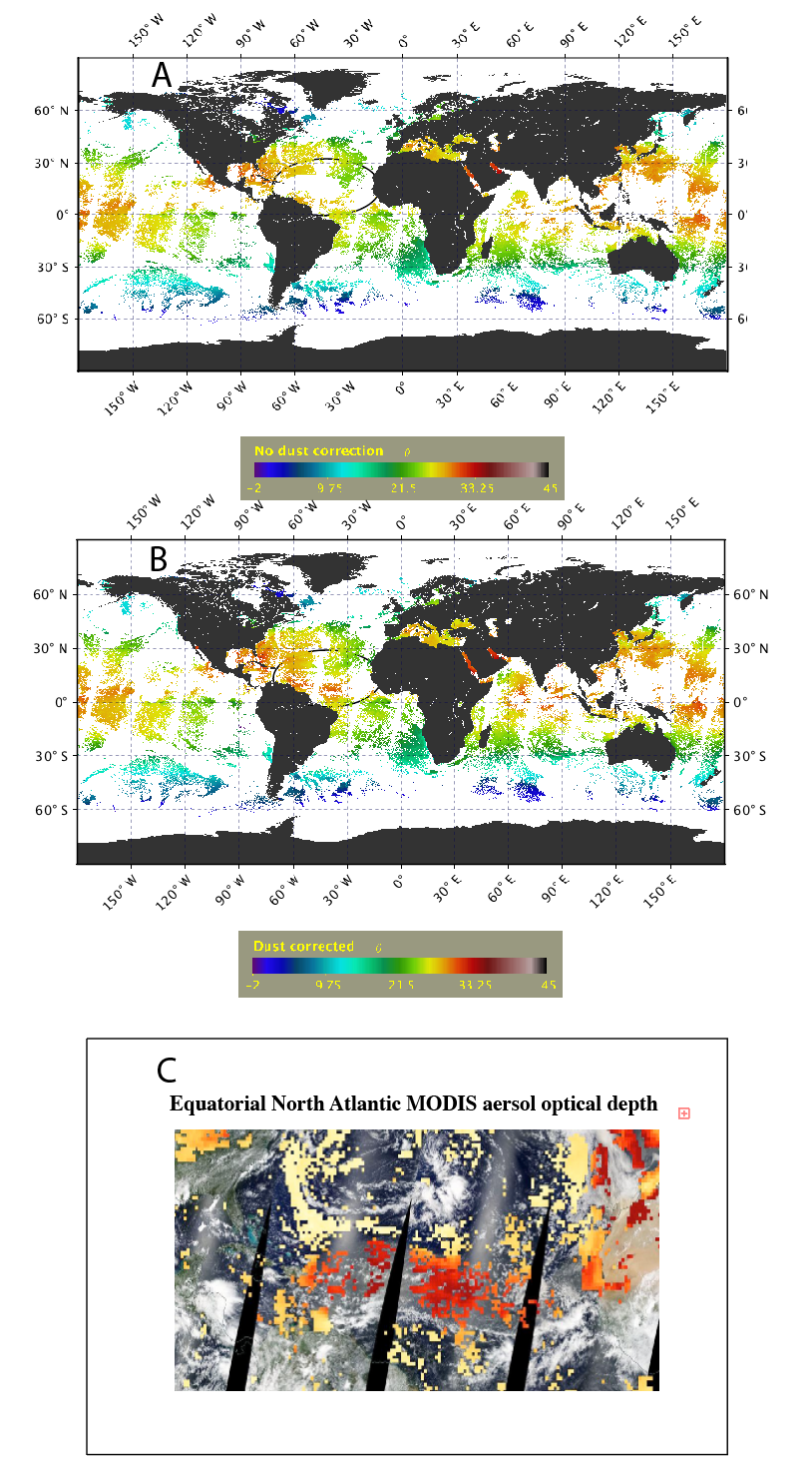
Beginning with MODIS R2019, a night time dust correction was implemented for the 11-12 μm night NSST product, as described by Luo et al. (2019). The correction uses a dust-induced SST difference index (DSDI), calculated from MODIS brightness temperatures measured in bands at infrared wavelengths of 3.8, 8.9, 10.8 and 12.0 μm, and the Modern-Era Retrospective Analysis for Research and Applications, Version 2 (MERRA-2; Gelaro et al., 2017) hourly dust extinction aerosol optical thickness (tavg1_2d_aer_Nx).
Using the DSDI correction increases the number of valid retrievals in the dust contaminated region of the equatorial and tropical North Atlantic Ocean. Figure 3 shows an L3 4 km image before and after the DSDI correction. The geographic area outlined by the black ellipse is an area predominantly flagged as bad due to dust contamination and excluded from the R2014 product. After the R2019 DSDI correction is applied there is a significant increase in the number of bins populated with high quality retrievals.
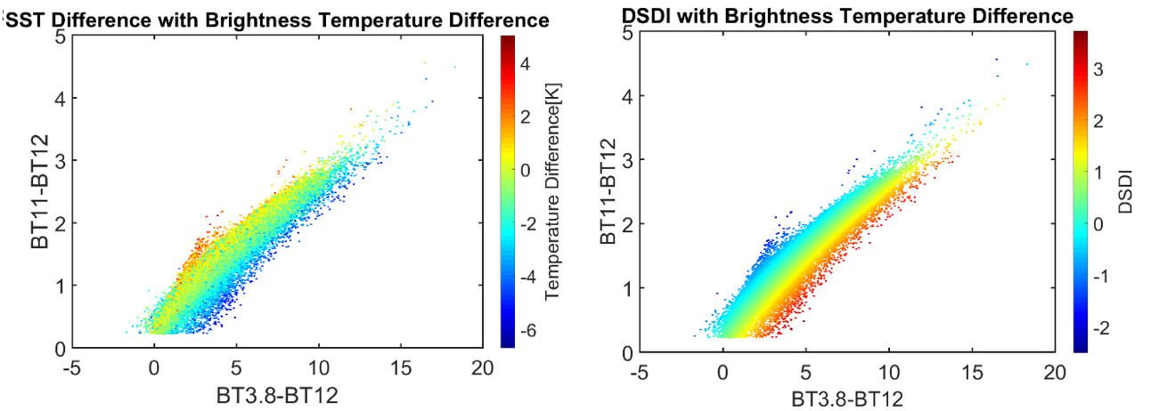
The coefficients for the DSDI were empirically derived using records from drifting buoys in the MODIS SST MUDB, from the North Atlantic between latitudes 0°N to 25°N and longitudes 40°W to 10°E. The matchup analysis was also augmented with infrared atmospheric radiative transfer simulations (RTTOV; Hocking et al. 2018) using data taken during six research cruises of the AEROSE program off West Africa, where there are frequent outflows of air containing Saharan Dust (Nalli et al. 2011). Figure 4 shows the relationships between the channel brightness temperature differences, temperature difference (MODIS – in situ SST), and the DSDI.
Principal component analysis (PCA) was used as an orthogonal transformation to convert the brightness temperature difference data into new linearly uncorrelated variables. As shown in Figure 5, the first Principal Component (PC) represents the greatest degree of variability in the SST dataset, which is the aerosol-free situation, and the deviation from the first PC of the BTs difference in the (BT3.8 - BT12 and BT11 - BT12) plane, which is the second axis of the remaining degree of variability, and can be used to represent the DSDI.

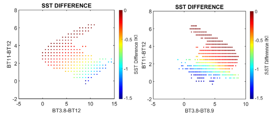
From the RTTOV model simulations (Figure 6), the aerosol free BT difference and the aerosol-contaminated BT difference relationship shows the difference is larger in the direction of increasing dust contaminations, so the simulations were used to establish the property, while the regression of BT difference and aerosol-introduced SST difference was used to determine the DSDI algorithms coefficients.
The DSDI index has the form:
\begin{align} DSDI= a + (b + c*S_{0}) * BT_{3.8} - BT_{12}) + (d + e*S_{0}) * (BT_{3.8} - BT_{8.9}) +\\ &\\ (f + g*S_{0}) * (BT_{11} - BT_{12}) + (h + i*S_0) * (BT_{11} - BT_{12})^2 + [a\sqrt{x} + \beta] \end{align}Where BT is the channel brightness temperature, S0 is the secant of the satellite zenith angle, x is the MERRA-2 dust extinction, and a:i, α and β are coefficients. The DSDI coefficients for R2019 processing are given in Table 4.
| DSDI Index Coefficients | MODIS AQUA | MODIS TERRA |
|---|---|---|
| a | 1.488 | 0.721 |
| b | 1.224 | 0.575 |
| c | -0.370 | -0.094 |
| d | 0.257 | -0.002 |
| e | 0.271 | 0.033 |
| f | -2.981 | -2.195 |
| g | -0.162 | 0.415 |
| h | -0.317 | 0.012 |
| i | 0.092 | -0.146 |
| alpha | 1.304 | 1.118 |
| beta | -0.107 | -0.009 |
The dust correction is only applied if both the daily MERRA-2 aerosol dust extinction is above 0.025 and the DSDI > 0.8. The magnitude of the applied correction is a linear function of the DSDI and has the form:
$$SST_{corrected} = SST + (j * DSDI + k)$$Regression coefficients j and k given in Table 5.
| Dust correction coefficients | AQUA | TERRA |
|---|---|---|
| j | 1.135 | 1.063 |
| k | -0.641 | -0.522 |
A day time flag for ice was introduced in VIIRS R2016.1 and MODIS R2019, based on 1.6 μm and 671 nm reflectances to reduce the misclassification of ice as open water during transitional ice conditions. The reflectance thresholds for this test were determined from spectral histograms of images manually classified as snow or ice from Sentinel-2 MSI calibrated reflectance (Hollstein et. al. 2016; see their Figure 1). This test is only evaluated at latitudes > 30° poleward of the sub-solar point, as the relative magnitudes of the reflectance can be impacted by sun glint.
The thresholds for the ice are:
$ρ(671 nm) > 0.3$ & $(0.1 > ρ(1.6 μm) ≥ 0.006)$Figure 7 shows an example of an L2 image from earlier VIIRS R2016.0 products of the thin/melting ice misclassification problem in the Arctic, and the impact of adding an additional test for ice to the cloud mask. The upper left panel of Figure 7 is a true color remapped L2 image. The large area outlined in red (A) has uniform appearance with different reflectance than its surroundings. The upper right panel shows pixels of good or better quality R2016 SST for the corresponding true color image. Area B highlights an area where ice was misclassified as clear open water. Retrievals over thin or melting ice can have temperatures close to those of open water, as shown in the unmasked SST L2 image on the lower left. In some conditions clouds or ice can even erroneously appear warmer than the open water, the yellow/green region in circle C is an area with temperatures of > 8°C. The cloud classification algorithms struggle in these conditions as it is assumed clouds or ice should be colder than the sea surface. The large overcorrection of ice and cloud top temperatures in polar regions is likely due to the regions of lower surface emissivity and the orientation of ice crystals in the atmosphere resulting in larger 11-12 μm BT differences (Vincent et al., 2008a, 2008b; Vincent 2019) than would be expected for the amount of water vapor present. Using the reflectance information from the 671 nm and 1.6 μm bands identifies when the cloud mask is likely to have misclassified an obscured pixel as clear.
Get Single Sensor Error Statistics for:
Get Nonlinear SST Coefficients for:
SST products are validated using a collocated matchup data base (MUDB) of in situ observations that are collected within 30 minutes of an overpass and 10 km of a pixel. The SST MUDB set is included in the SEABASS archive. The in situ data sources include both sub-surface in situ observations from drifting and fixed buoy downloaded from the NOAA in situ SST quality monitor (iQuam; Xu and Ignatov 2014), and direct measurements of ocean skin temperatures from ship board Marine-Atmospheric Emitted Radiance Interferometer (M-AERI; Minnett et al. 2001). The M-AERI validation provides SI traceability to standards at NIST (National Institute of Standards and Technology; Rice et al. 2004) and NPL (National Physical Laboratory, UK; Theocharous et al., 2019). However, the quantity and geographical coverage of radiometer skin SST measurements are significantly less than large network of buoy subsurface temperature measurements, but which have a larger calibration uncertainty.
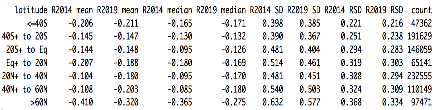
The multi-dimensional single sensor error statistics (SSES) look-up tables of bias error and uncertainty relative to buoy measurements have been updated based on the R2019 validation results. The bias and uncertainty SSES in the GHSST L2P files are a function of quarter of year, latitude band, satellite zenith angle, brightness temperature difference intervals, temperature intervals, and quality level. Tables 6 and 7 summarize the global statistics of the highest quality retrievals as a function of latitude for both the current R2014 and R2019.
 |
 |
| Residuals sensor skin SST – sub-surface buoy SST |
|||||||
|---|---|---|---|---|---|---|---|
| Sensor | quality | mean | median | SD | RSD | Count | |
| TERRA SST | 0 | -0.166 | -0.150 | 0.442 | 0.319 | 538918 | |
| AQUA SST | 0 | -0.185 | -0.170 | 0.423 | 0.305 | 508950 | |
| VIIRS SST | 0 | -0.205 | -0.174 | 0.476 | 0.343 | 473498 | |
| TERRA SST | 1 | -0.424 | -0.395 | 0.641 | 0.462 | 252809 | |
| AQUA SST | 1 | -0.424 | -0.380 | 0.620 | 0.447 | 267214 | |
| VIIRS SST | 1 | -0.451 | -0.377 | 0.730 | 0.527 | 223565 | |
| Residuals sensor skin SST – skin radiometer SST |
|||||||
|---|---|---|---|---|---|---|---|
| Sensor | quality | mean | median | SD | RSD | Count | |
| TERRA SST | 0 | -0.058 | -0.052 | 0.481 | 0.347 | 3069 | |
| AQUA SST | 0 | 0.042 | 0.040 | 0.494 | 0.347 | 2070 | |
| VIIRS SST | 0 | 0.030 | 0.009 | 0.196 | 142 | 81 | |
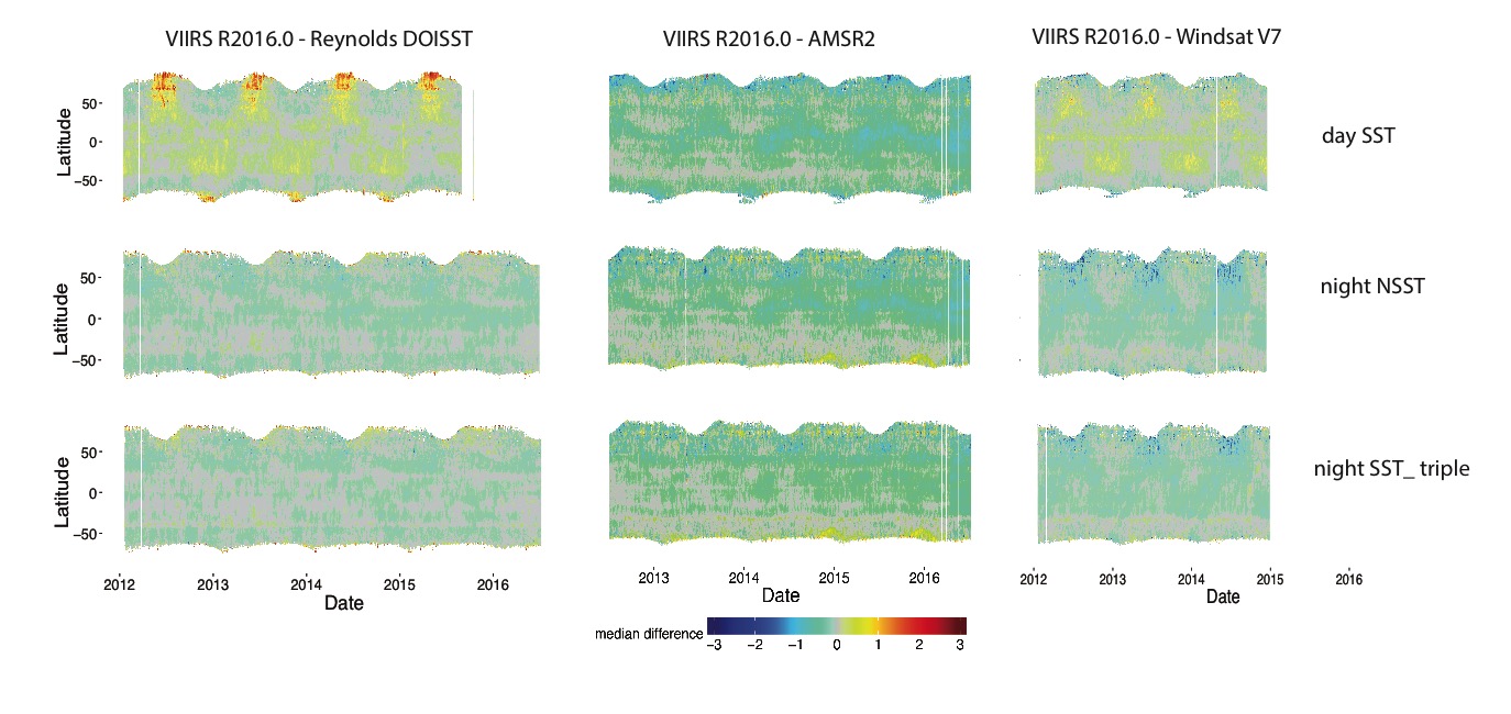
Comparisons between VIIRS R2016.0 skin SSTs composites of WindSat SSTs, AMSRE, and Daily Reynolds DOI fields are shown in Figure 11 as Hovmoller plots of the 4km zonal average differences.
Banzon, V.F., Reynolds, R.W., Stokes, D., & Xue, Y. (2014). A 1/4°-Spatial-Resolution Daily Sea Surface Temperature Climatology Based on a Blended Satellite and in situ Analysis. Journal of Climate 27, 8221-8228. doi: 10.1175/JCLI-D-14-00293.1.
Banzon, V., Smith, T.M., Chin, T.M., Liu, C., & Hankins, W. (2016). A long-term record of blended satellite and in situ sea-surface temperature for climate monitoring, modeling and environmental studies. Earth Syst. Sci. Data 8, 165-176. doi: 10.5194/essd-8-165-2016.
Bernhard, P., Holmes, G., & Kirkby, R. (2001). Optimizing the Induction of Alternating Decision Trees. Proceedings of the Fifth Pacific-Asia Conference on Advances in Knowledge Discovery and Data Mining (2001), Advances in Knowledge Discovery and Data Mining, pp. 477-487.
Brasnett B., (2008). The impact of satellite retrievals in a global sea-surface-temperature analysis. Q.J.R. Meteorol. Soc., 134, 1745-1760. doi: 10.1002/qj.319
Breiman, L., Friedman, J., Stone, C.J., & Olshen, R.A. (1984). Classification and regression trees. (pp. 358) Boca Raton, FL, USA.: Chapman and Hall/CRC press. ISBN: 0412048418.
Brown, O.B. & Minnett, P.J. (1999). MODIS Infrared Sea Surface Temperature Algorithm — Algorithm Theoretical Basis Document. University of Miami. 91 pp.
Corlett, G.K., Merchant, C.J., Minnett, P.J., & Donlon, C.J. (2014). Assessment of Long-Term Satellite Derived Sea Surface Temperature Records. In G. Zibordi, C.J. Donlon, & A.C. Parr (Eds.), Experimental Methods in the Physical Sciences, Vol 47, Optical Radiometry for Ocean Climate Measurements (pp. 639-677): Academic Press. 1079-4042. doi: 10.1016/B978-0-12-417011-7.00021-0.
Donlon, C.J., Robinson, I., Casey, K.S., Vazquez-Cuervo, J., Armstrong, E., Arino, O., Gentemann, C., May, D., Le Borgne, P., Piollé, J., Barton, I., Beggs, H., Poulter, D.J.S., Merchant, C.J., Bingham, A., Heinz, S., Harris, A., Wick, G., Emery, B., Minnett, P., Evans, R., Llewellyn-Jones, D., Mutlow, C., Reynolds, R.W., Kawamura, H., & Rayner, N. (2007). The Global Ocean Data Assimilation Experiment High-resolution Sea Surface Temperature Pilot Project. Bulletin of the American Meteorological Society 88, 1197-1213.
Freund, Y., Mason, L. (1999). The Alternating Decision Tree Learning Algorithm. In Proceedings of the Sixteenth International Conference on Machine Learning (ICML '99), Ivan Bratko and Saso Dzeroski (Eds.). Morgan Kaufmann Publishers Inc., San Francisco, CA, USA, 124-133.
Gelaro, R., McCarty, W., Suárez, M.J., Todling, R., Molod, A., Takacs, L., Randles, C.A., Darmenov, A., Bosilovich, M.G., Reichle, R., Wargan, K., Coy, L., Cullather, R., Draper, C., Akella, S., Buchard, V., Conaty, A., da Silva, A.M., Gu, W., Kim, G.-K., Koster, R., Lucchesi, R., Merkova, D., Nielsen, J.E., Partyka, G., Pawson, S., Putman, W., Rienecker, M., Schubert, S.D., Sienkiewicz, M., & Zhao, B. (2017). The Modern-Era Retrospective Analysis for Research and Applications, Version 2 (MERRA-2). Journal of Climate 30, 5419-5454. doi: 10.1175/jcli-d-16-0758.1
Hanafin, J. A. (2002). On sea surface properties and characteristics in the infrared. Thesis (Ph.D.) University of Miami, 2002.; Publication Number: AAI3056632; ISBN: 9780493717869; Source: Dissertation Abstracts International, Volume: 63-06, Section: B, page: 2767.; 111 p.
Hanafin, J. A. & P. J. Minnett (2003). Profiling temperature in the sea surface skin layer using FTIR measurements. Gas Transfer at Water Surfaces. edited by M. A. Donelan, W. M. Drennan, E. S. Saltzmann and R. Wanninkhof. American Geophysical Union Monograph 127, 161-166
Hocking, J., Rayer, P., Rundle, D., Saunders, R., Matricardi, M., Geer, A., Brunel, P., & Vidot, J. (2018). RTTOV v12 Users Guide, EUMETSAT Satellite Application Facility on Numerical Weather Prediction (NWP SAF), (142 pp.): EUMETSAT. Available here.
Hollstein, A., Segl, K., Guanter, L., Brell, M., & Enesco, M. (2016). Ready-to-Use Methods for the Detection of Clouds, Cirrus, Snow, Shadow, Water and Clear Sky Pixels in Sentinel-2 MSI Images. Remote Sensing 8, 666.2072-4292, Available here.
Jia, C. (2019). Satellite Infrared Retrievals of Sea Surface Temperature at High Latitudes. MS Thesis, Meteorology and Physical Oceanography. University of Miami. Miami. FL, USA. pp. 79. Available here.
Jia, C., & Minnett, P.J. (2020). High Latitude Sea Surface Temperatures Derived from MODIS Infrared Measurements Remote Sensing of Environment. In review.
Kilpatrick, K. A. Podestá, G.P., & Evans, R.H. (2001). Overview of the NOAA/NASA advanced very high resolution radiometer Pathfinder algorithm for sea surface temperature and associated matchup database. Journal of Geophysical Research. 106(C5):9179-9197. doi: 10.1029/1999JC000065
Kilpatrick, K. A., G. Podestá, S. Walsh, E. Williams, V. Halliwell, M. Szczodrak, O. B. Brown, P. J. Minnett, and R. Evans (2015). A decade of sea surface temperature from MODIS. Remote Sensing of Environment, 165, 27-41. doi: 10.1016/j.rse.2015.04.023
Kilpatrick, K. A., G. Podestá, E. Williams, S. Walsh, & P. J. Minnett, (2019a): Alternating Decision Trees for Cloud Masking in MODIS and VIIRS NASA Sea Surface Temperature Products. J. Atmos. Oceanic Technol., 36, 387–407, doi: 10.1175/JTECH-D-18-0103.1
Kilpatrick, K. A., P. Minnett, B. Luo, (2019b). Validation of NASA MODIS R2019.0 reprocessed SST Products. The 18th International GHRSST Science Team Meeting (GHRSST XVIII) – Frascati Italy- 6th to 10th June 2019.
Liang, X., & Ignatov, A. (2013). AVHRR, MODIS, and VIIRS radiometric stability and consistency in SST bands. J. Geophys. Res. Oceans, 118(6), 3161–3171. doi: 10.1002/jgrc.20205
Liu, C., E. Freeman, E. C. Kent, B. Huang, H. M. Zhang, D. I. Berry, S. J. Worley, M. Ouellet, I. Gaboury, Z. Li, & V.F. Banzon (2019). ICOADS Drifting Buoy Data Recovery from BUFR and Its Impact on the OISST and ERSST. Poster presentation. American Meteorological Society 99th annual Meeting, Phoenix, January 6-10 2019. Available here.
Liu, Y., & Minnett, P.J. (2016). Sampling errors in satellite-derived infrared sea-surface temperatures. Part I: Global and regional MODIS fields. Remote Sensing of Environment 177, 48-64. doi: 10.1016/j.rse.2016.02.026.
Liu, Y., Chin, T.M., & Minnett, P.J. (2017). Sampling errors in satellite-derived infrared sea-surface temperatures. Part II: Sensitivity and parameterization. Remote Sensing of Environment 198, 297-309. doi: 10.1016/j.rse.2017.06.011
Luo, B. (2018). Improving Satellite Retrieved Infrared Sea Surface Temperatures in Aerosol Contaminated Regions. MS Thesis, Meteorology & Physical Oceanography. University of Miami. 2018. pp. 75. Available here.
Luo, B., Minnett, P. J., Gentemann, C. and Szczodrak, G. (2019). Improving satellite retrieved night-time infrared sea surface temperatures in aerosol contaminated regions, Remote Sensing of Environment, 223, doi: 10.1016/j.rse.2019.01.009
Merchant, C.J., Harris, A.R., Maturi, E. & MacCallum, S. (2005). Probabilistic physically based cloud screening of satellite infrared imagery for operational sea surface temperature retrieval. Quarterly Journal of the Royal Meteorological Society, 131: 2735-2755.
Minnett, P.J. (2003). Radiometric measurements of the sea-surface skin temperature - the competing roles of the diurnal thermocline and the cool skin. International Journal of Remote Sensing 24, 5033-5047.
Minnett, P. J. (2010). The Validation of Sea Surface Temperature Retrievals from Spaceborne Infrared Radiometers. Oceanography from Space, revisited., V. Barale, J. F. R. Gower, and L. Alberotanza, Eds., Springer Science+Business Media B.V., 229-247.
Minnett, P. J., & G. K. Corlett (2012). A pathway to generating Climate Data Records of sea-surface temperature from satellite measurements. Deep Sea Research Part II: Topical Studies in Oceanography 77 (2012): 44-51.
Minnett, P. J., Evans, R. H., Podestá, G. P., & Kilpatrick, K. A. (2014). Sea-surface temperature from Suomi-NPP VIIRS: Algorithm development and uncertainty estimation. In Proceedings of SPIE - The International Society for Optical Engineering. (Vol. 9111). [91110C] SPIE.
Nalli, N.R., Joseph, E., Morris, V.R., Barnet, C.D., Wolf, W.W., Wolfe, D., Minnett, P.J., Szczodrak, M., Izaguirre, M.A., Lumpkin, R., Xie, H., 2011. Multiyear observations of the tropical Atlantic atmosphere: multidisciplinary applications of the NOAA aerosols and ocean science expeditions. Bull. Am. Meteorol. Soc. 92 (6), 765–789.
Pfahringer, B., G. Holmes, & R. Kirkby (2001). Optimizing the induction of alternating decision trees. Fifth Pacific-Asia Conf. on Advances in Knowledge Discovery and Data Mining, Hong Kong, China, PAKDD, 477–487, Available at http://www.cs.waikato.ac.nz/ml/publications/2001/pakdd2001.pdf.
Reynolds, Richard W., Thomas M. Smith, Chunying Liu, Dudley B. Chelton, Kenneth S. Casey, Michael G. Schlax, 2007: Daily High-Resolution-Blended Analyses for Sea Surface Temperature. J. Climate, 20, 5473-5496.
Rice, J.P., Butler, J.J., Johnson, B.C., Minnett, P.J., Maillet, K.A., Nightingale, T.J., Hook, S.J., Abtahi, A., Donlon, C.J., & Barton, I.J. (2004). The Miami2001 Infrared Radiometer Calibration and Intercomparison: 1. Laboratory Characterization of Blackbody Targets. Journal of Atmospheric and Oceanic Technology 21, 258-267.
Theocharous, E., Fox, N.P., Barker-Snook, I., Niclòs, R., Santos, V.G., Minnett, P.J., Göttsche, F.M., Poutier, L., Morgan, N., Nightingale, T., Wimmer, W., Høyer, J., Zhang, K., Yang, M., Guan, L., Arbelo, M., & Donlon, C.J. (2019). The 2016 CEOS Infrared Radiometer Comparison: Part II: Laboratory Comparison of Radiation Thermometers. Journal of Atmospheric and Oceanic Technology 36, 1079-1092. doi: 10.1175/jtech-d-18-0032.1
Vincent, R. (2019). The Case for a Single Channel Composite Arctic Sea Surface Temperature Algorithm. Remote Sens. 2019, 11, 2393.
Vincent, R.F., Marsden, R.F., Minnett, P.J., Creber, K.A.M., & Buckley, J.R. (2008a). Arctic Waters and Marginal Ice Zones: A Composite Arctic Sea Surface Temperature Algorithm using Satellite Thermal Data. Journal of Geophysical Research 113, C04021. doi: 10.1029/2007JC004353
Vincent, R.F., Marsden, R.F., Minnett, P.J., & Buckley, J.R. (2008b). Arctic Waters and Marginal Ice Zones: Part 2 - An Investigation of Arctic Atmospheric Infrared Absorption for AVHRR Sea Surface Temperature Estimates. Journal of Geophysical Research 113, C08044. doi: 10.1029/2007JC004354
Walton, C. C., Pichel, W. G., Sapper, J. F., and May, D. A. (1998). The development and operational application of nonlinear algorithms for the measurement of sea surface temperatures with the NOAA polar-orbiting environmental satellites, Journal of Geophysical Research, 103(C12), 27999–28012, doi: 10.1029/98JC02370.
Ward, B. (2006). Near-Surface Ocean Temperature. Journal of Geophysical Research 111, C02005. doi: 10.1029/2004JC002689
Wong, E.W., & Minnett, P.J. The Response of the Ocean Thermal Skin Layer to Variations in Incident Infrared Radiation. Journal of Geophysical Research: Oceans, 123, 19pp. doi: 10.1002/2017JC013351
Xu, F., & Ignatov, A. (2014). In situ SST Quality Monitor (iQuam). Journal of Atmospheric and Oceanic Technology 31, 164-180. doi: 10.1175/JTECH-D-13-00121.1
