The aerosol correction algorithm utilizes two bands either in the NIR or SWIR spectral range by calculating a band ratio of the Rayleigh, surface, and gas corrected reflectance, namely epsilon, as follows:
$$\varepsilon = \frac{\rho_a(\lambda_s)}{\rho_a(\lambda_l)}$$ ,where $\lambda_s$ and $\lambda_l$ correspond to the short and long wavelength either in the NIR or SWIR range (e.g. for MODIS $\lambda_s$=748 nm and $\lambda_l$=869 nm) and \rho_a(\lambda) is the aerosol reflectance defined as:
$$\rho_a(\lambda) = \frac{\pi \times [L_a(\lambda)+L_{ra}(\lambda)]}{F_0 \times \mu_0}$$$F_0$ is the extraterrestrial solar irradiance and $\mu_0$ is the cosine of the solar zenith angle. The normalization removes the geometry dependence; however, the aerosol radiance term is a strong function of the viewing geometry, thus the LUT is generated as a function of the solar and sensor zenith angle and relative azimuth angle.
NASA’s previous approach to estimate the aerosol reflectance term is by finding the best match of the observed epsilon value to the LUT. Here epsilon is calculated using the single scattering aerosol reflectance at two NIR/SWIR bands. Since the LUT is calculated for a set of deterministic aerosol models based on Ahmad et al., 2010, the algorithm interpolates the single scattering aerosol reflectance from the LUT to match the observed reflectance. However, the single scattering assumption is not valid for an optically thick atmosphere where the Rayleigh optical depth is increasing with $\lambda^{-4}$ at short wavelengths. Accounting for multiple scattering interaction between the aerosol and molecules and between aerosols is crucial when extrapolating the reflectance to short wavelengths. Given the aerosol type estimated from the epsilon, the single scattering aerosol reflectance in short wavelengths are extrapolated from that in one NIR/SWIR wavelength and then are used to estimate the corresponding multiple scattering aerosol reflectance through a polynomial relationship derived through vector radiative transfer simulations (Gordon and Wang, 1994). The multiple scattering aerosol reflectance is then used for the aerosol correction.
NASA’s new approach to the aerosol determination is called the multi-scattering Epsilon or (MSEPS) outlined in Ahmad and Franz (2018) and has been utilized in the multi-band atmospheric correction algorithm (MBAC) (Ibrahim et al, 2019). The aerosol model and optical properties determination is done in multiple scattering space. It is based on the Ahmad et al. (2010) aerosol models, for which the top of atmosphere (TOA) reflectance due to aerosols can be described by three parameters: relative humidity (RH), Angstrom exponent ($\alpha$) or the analogous fine-mode fraction (f), and optical thickness of the aerosols ($\tau$) in the model atmosphere. Briefly, for any relative humidity suite, the dependence of multiple-scattering-epsilon $\varepsilon(λ)=(\rho(\lambda))⁄(\rho(\lambda_l))$ on $\rho(\lambda_l)$ would look like the x-y plot shown in Figure 1 for MODISA as an example, where $\rho_l$ = 869nm. Here, $\rho$ refers to TOA aerosol reflectance and the subscript numbers refer to wavelength bands.
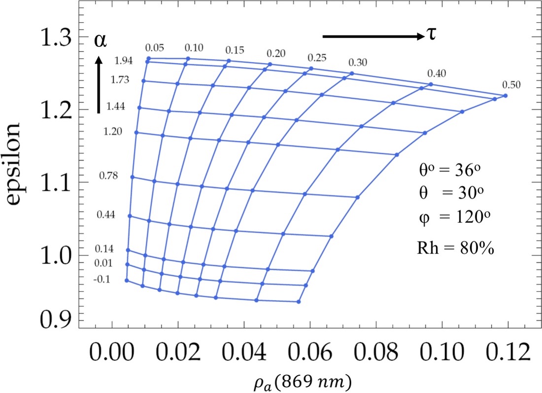
In the above figure, the aerosol optical depth ($\tau$) varies along the ‘horizontal’ axis, and the Angstrom exponent ($\alpha$), and extinction coefficients ($\xi$) vary along the ‘vertical’ axis. This parametrization of the LUT allows to readily calculate the aerosol reflectance at any grid point. One advantage of this approach over the current NASA standard algorithm is that it provides a mathematical formulation for the aerosol reflectance determination that facilitates the application of standard error propagation techniques.
The aerosol reflectance at each wavelength > 800 nm is stored in a LUT as a quadratic polynomial function of the aerosol optical depth, relative humidity, and fine mode fraction:
$$\rho_a (\lambda,\tau_a,RH,f)=a(\lambda,RH,f)+b(\lambda,RH,f)\times\tau_a+c(\lambda,RH,f)\times\tau_a^2,$$where a, b, and c are the fitting coefficients stored in the aerosol LUT. For any spectral band in the NIR-SWIR range at which the water-leaving radiance can be assumed negligible in open ocean conditions or non-negligible in turbid conditions where the NIR water-leaving radiance can be estimated using Bailey et. al, 2010. Assuming a proper correction for absorbing gases and Rayleigh (+ surface) scattering has been done, aerosol reflectance at a NIR/SWIR band can be determined and the aerosol optical depth can then be estimated by solving the quadratic equation, as:
$$\tau_a (\lambda=\lambda_l,RH,f) = \frac{(0.5 \times [-b(\lambda_l,RH,f)]) + \sqrt{b(\lambda_l,RH,f)^2-4 \times (a - \rho_a^{obs}(\lambda_l)})}{c(\lambda_l,RH,f)}$$For consistency with the system vicarious calibration procedure, which is performed relative to one wavelength in the NIR (e.g. 869 nm for MODIS), the optical depth is estimated at that wavelength.
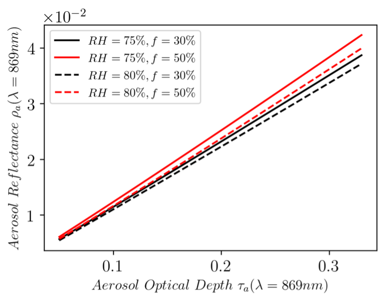
For an observed aerosol reflectance, the optical depth can be calculated for each aerosol model set (RH,f) as shown in Figure 2 as an example for MODISA within a relative humidity bracket from the ancillary field.
The algorithm then reevaluates the aerosol optical depth and reflectance spectrally for all aerosol models within each relative humidity bracket, as:
$$\tau_a (\lambda,RH,f)=\xi(\lambda,RH,f)/\xi(\lambda_l,RH,f) \times\tau_a (\lambda_l,RH,f)$$ ,where $\xi(\lambda,RH,f)$ is the aerosol extinction coefficient. Then, the spectral aerosol reflectance for each aerosol model set (RH,f) is recalculated from the polynomial equation above to estimate the aerosol reflectance at the short NIR wavelength, $\lambda_s$.
Given the aerosol reflectance at both the NIR wavelengths ($\lambda_l,\lambda_s$), the multi-scattering epsilon is calculated for each of the two relative humidity sets for the 10 fine mode fractions. In a similar approach to Gordon and Wang 1994, the observed epsilon is compared to the model to find the appropriate weight of the bracketing models when mixed (i.e., linear mixing). Once the best mixed models are obtained within each humidity set, the same linear mixing approach is done to find the mixed aerosol reflectance across the relative humidity dimension, where the weight is obtained from the observed humidity coming from ancillary source as follows:
$$\rho_a (\lambda,RH_{obs},f_{mix} )= (1-w_{RH})\times\rho_a (\lambda,RH_1,f_{mix} )+w_{RH}\times\rho_a (λ,RH_2,f_{mix})$$The final $\rho_a (\lambda,RH_{obs},f_{mix})$ should match the TOA aerosol reflectance observations in the NIR channels, while the extrapolated reflectance to the visible channels based on the model mixtures are used for the aerosol correction using the 4th order polynomial equation below:
$$\rho_a (\lambda,\tau_a,RH,f)=a(\lambda,RH,f)+b(\lambda,RH,f)\times\tau_a+c(\lambda,RH,f)\times\tau_a^2+d(\lambda,RH,f)\times\tau_a^3+e(\lambda,RH,f)\times\tau_a^4$$where the coefficients a, b, c, d, and e are stored in a LUT. Given the fine-mode fraction weight, the relative humidity weight, and the aerosol optical depth, the diffuse transmittance of the atmosphere can then be evaluated similarly.
Ahmad, Ziauddin, Bryan A. Franz, Charles R. McClain, Ewa J. Kwiatkowska, Jeremy Werdell, Eric P. Shettle, and Brent N. Holben. 2010. “New Aerosol Models for the Retrieval of Aerosol Optical Thickness and Normalized Water-Leaving Radiances from the SeaWiFS and MODIS Sensors over Coastal Regions and Open Oceans.” Applied Optics 49 (29): 5545. https://doi.org/10.1364/AO.49.005545.
Ahmad, Ziauddin, and Bryan A. Franz (2018), Uncertainty in aerosol model characterization and its impact on ocean color retrievals, in PACE Technical Report Series, Volume 6: Data Product Requirements and Error Budgets (NASA/TM-2018 – 2018-219027/ Vol. 6), edited by I. Cetinić, C. R. McClain and P. J. Werdell, NASA Goddard Space Flight Space Center Greenbelt, MD.
Bailey, Sean W., Bryan A. Franz, and P. Jeremy Werdell. 2010. “Estimation of near-Infrared Water-Leaving Reflectance for Satellite Ocean Color Data Processing.” Optics Express 18 (7): 7521. https://doi.org/10.1364/OE.18.007521.
Gordon, Howard R., and Menghua Wang. 1994. “Retrieval of Water-Leaving Radiance and Aerosol Optical Thickness over the Oceans with SeaWiFS: A Preliminary Algorithm.” Applied Optics 33 (3): 443. https://doi.org/10.1364/AO.33.000443.
Ibrahim, Amir, Franz, Bryan A., Ahmad, Ziauddin. and Bailey, Sean W., 2019. Multiband atmospheric correction algorithm for ocean color
